pip install mne
pip install braindecode
pip install mne_bids
pip install --upgrade mne-bids-pipeline
pip install numpy matplotlib scipy numba scikit-learn mne PyWavelets pandas
pip install mne-featuresThis Project at a Glance
In this project, I step into the amazing world of neuroscience and apply machine learning methodologies to predict an individual’s age using electroencephalogram (EEG) data. The prediction pipeline involves feature extraction, engineering, selection, and finally, predictive modeling. The ultimate goal of this project is to examine how accurately we can predict a person’s age using EEG data.
Dataset Information
The project uses a dataset available on OpenNeuro (Accession Number ds003775), authored by Christoffer Hatlestad-Hall, Trine Waage Rygvold, and Stein Andersson. The dataset, updated on November 23, 2022, features electroencephalogram (EEG) data for 111 participants spanning two sessions.
You can find more about the dataset here.
Approaches Used
I used two approaches in this project: one using handcrafted features with machine learning models, and another leveraging deep learning. In both approaches, I used the MNE_BIDS Pipeline for processing and analyzing the EEG data. This pipeline follows the Brain Imaging Data Structure (BIDS) standard, ensuring consistency and accessibility of data and metadata for further analysis.
To install the necessary dependencies, run the following code:
Approach 1: Handcrafted Features and Machine Learning Models
Handcrafted features approach emphasizes on the utilization of a-priori defined features, which are inspired by theoretical and empirical results in neuroscience and neural engineering.
Feature Extraction
The feature extraction was performed using a script named feature_extraction.py. It loads each participant’s EEG data, computes a set of predefined features (inspired by theoretical and empirical results in neuroscience and neural engineering), and appends these features to a DataFrame.
# Code snippet from feature_extraction.py

from mne_features.feature_extraction import extract_features
import mne
from joblib import Parallel, delayed
import pandas as pd

def compute_features(i, ch_name, epochs):
    ch_data = epochs.get_data(picks=ch_name)
    features = extract_features(ch_data, sfreq=epochs.info['sfreq'], selected_funcs=selected_funcs, funcs_params=selected_params, return_as_df=False)
    feature_dict = {}
    for feature_name, feature_values in zip(selected_funcs, features):
        feature_dict[f'{ch_name}_{feature_name}'] = feature_values[0]
    return feature_dict
And the second part:
def main():
    feature_df = pd.DataFrame()
    participants = pd.read_csv('../participants.tsv', sep='\t')
    subject_ids = participants['participant_id'].unique()
    frequency_bands = [0, 2, 4, 8, 13, 18, 24, 30, 49]
    selected_funcs = [
        'mean', 'std', 'kurtosis', 'skewness', 'quantile', 'ptp_amp',
        'pow_freq_bands', 'spect_entropy', 'app_entropy', 'samp_entropy',
        'hurst_exp', 'hjorth_complexity', 'hjorth_mobility', 'line_length',
        'wavelet_coef_energy', 'higuchi_fd', 'zero_crossings', 'svd_fisher_info'
    ]
    selected_params = {
        'quantile__q': [0.1, 0.25, 0.75, 0.9],
        'pow_freq_bands__freq_bands': frequency_bands,
    }

    for sub_id in subject_ids:
        epochs = mne.read_epochs(f'../derivatives/{sub_id}/ses-t1/eeg/{sub_id}_ses-t1_task-resteyesc_proc-clean_epo.fif')
        results = Parallel(n_jobs=-1, backend='loky')(delayed(compute_features)(i, ch_name, epochs) for i, ch_name in enumerate(epochs.ch_names))
        feature_dict = {}
        for result in results:
            feature_dict.update(result)
        subject_age = participants.loc[participants['participant_id'] == sub_id, 'age'].values[0]
        feature_dict['age'] = subject_age
        feature_df = feature_df.append(pd.DataFrame(feature_dict, index=[0]), ignore_index=True)
        feature_df.to_csv('feature_df.csv', index=False)
if __name__ == "__main__":
    main()
Exploratory Data Analysis
After feature extraction, I performed an exploratory data analysis. First, I plotted the distribution of the target variable, ‘age’. Then, I computed summary statistics for the features and checked for missing values.
import matplotlib.pyplot as plt
import seaborn as sns

# Set the style
sns.set(style="whitegrid")

# Plot the distribution of the target variable 'age'
sns.displot(df['age'], kde=True)
plt.title('Distribution of Age')
plt.show()

# Print summary statistics of the features
print(df.describe())

# Check for missing values
missing_values = df.isnull().sum().sum()
print(f"Number of missing values in the dataset: {missing_values}")
print(f"Shape of the dataset: {df.shape}")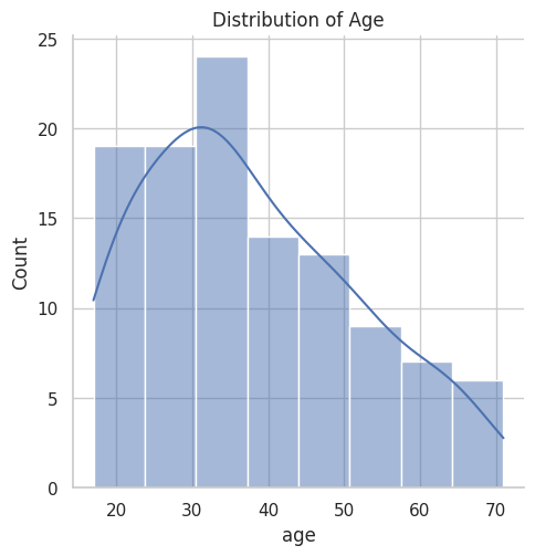
Feature Selection
To narrow down the number of features for the machine learning models, I used the SelectKBest class from the sklearn.feature_selection module. This class scores the features based on a function, in this case, the mutual information with the target variable ‘age’, and selects the top ‘k’ features.
from sklearn.feature_selection import SelectKBest, mutual_info_regression

# Select the top k features based on their mutual information with the target variable 'age'
selector = SelectKBest(mutual_info_regression, k=100)

# Fit the selector to the data
X = df.drop('age', axis=1)
y = df['age']
selector.fit(X, y)

# Get the indices of the selected features
selected_features = selector.get_support(indices=True)

# Create a new df with only the selected features
selected_df = df.iloc[:,selected_features]

# Add the target variable 'age' to this df
selected_df['age'] = df['age']

# Show the selected features
selected_df.head()
Dimensionality Reduction
Next, I applied Principal Component Analysis (PCA) for further dimensionality reduction. Before that, I scaled the features using StandardScaler from the sklearn.preprocessing module. PCA was used to create a smaller number of uncorrelated variables that still contained most of the information in the original dataset.
from sklearn.decomposition import PCA
from sklearn.preprocessing import StandardScaler

selected_df = selected_df.copy()

# Scale the features
scaler = StandardScaler()
scaled_features = scaler.fit_transform(selected_df.drop('age', axis=1))

# Apply PCA
pca = PCA(n_components=4)
pca_features = pca.fit_transform(scaled_features)

# Add the PCA components to the original df
for i in range(pca_features.shape[1]):
    selected_df[f'PC{i+1}'] = pca_features[:, i]

selected_df.shape
Model Comparison
For the initial model comparison, I used a variety of machine learning models and compared their performance using 5-fold cross-validation. The performance metric used was the Mean Absolute Error (MAE), which is the average of the absolute differences between the predicted and actual values.
from sklearn.dummy import DummyRegressor
from sklearn.model_selection import cross_val_score, KFold
from sklearn.linear_model import LinearRegression, Ridge, Lasso, ElasticNet
from sklearn.ensemble import RandomForestRegressor, AdaBoostRegressor, GradientBoostingRegressor
from xgboost import XGBRegressor
from sklearn.svm import SVR
from sklearn.tree import DecisionTreeRegressor
import numpy as np

def compare_models(df):
    # Define models
    models = [
        ("Dummy", DummyRegressor(strategy="mean")),
        ("Linear Regression", LinearRegression()),
        ("Ridge Regression", Ridge(random_state=42)),
        ("Lasso Regression", Lasso(random_state=42)),
        ("ElasticNet", ElasticNet(random_state=42)),
        ("Random Forest", RandomForestRegressor(random_state=42)),
        ("AdaBoost", AdaBoostRegressor(random_state=42)),
        ("GradientBoosting", GradientBoostingRegressor(random_state=42)),
        ("XGBoost", XGBRegressor(random_state=42)),
        ("SVM", SVR()),
        ("Decision Tree", DecisionTreeRegressor(random_state=42))
    ]

    # Define features and target
    X = df.loc[:, df.columns != 'age']
    y = df['age']

    # Initialize an empty fd to store the results
    results_df = pd.DataFrame(columns=["model", "MAE"])

    # Apply 5-fold cv and store MAE
    for model_name, model in models:
        kfold = KFold(n_splits=5, random_state=42, shuffle=True)
        mae = cross_val_score(model, X, y, cv=kfold, scoring='neg_mean_absolute_error')
        results_df = pd.concat([results_df, pd.DataFrame({"model": [model_name], "MAE": [-mae.mean()]})], ignore_index=True)

    # Sort the df by MAE
    results_df = results_df.sort_values(by="MAE", ascending=True)

    def highlight_rows(row):
        if row['model'] == 'Dummy':
            return ['background-color: red']*2
        else:
            return ['background-color: white']*2

    # Return the styled df
    return results_df.style.apply(highlight_rows, axis=1)

# Use the function
compare_models(selected_df)| Model | MAE |
|---|---|
| SVM | 11.165101 |
| ElasticNet | 11.319560 |
| Ridge Regression | 11.334589 |
| Lasso Regression | 11.342098 |
| Dummy | 11.659533 |
| Random Forest | 12.188336 |
| AdaBoost | 12.342140 |
| GradientBoosting | 12.963295 |
| XGBoost | 13.344670 |
| Decision Tree | 16.696443 |
| Linear Regression | 38.469241 |
Hyperparameter Tuning
After identifying the top-performing models, I used GridSearchCV from the sklearn.model_selection module to find the optimal hyperparameters for each model. This exhaustive search on a specified parameter grid returns the combination of parameters that gives the best performance.
from sklearn.model_selection import GridSearchCV

# Define the hyperparameters to search for each model
hyperparameters = {
    "AdaBoost": {
        "n_estimators": [2, 3, 5, 10, 25, 50, 75, 100, 150, 200],
        "learning_rate": [0.001, 0.01, 0.1, 1.0]
    },

    "SVM": {
        "C": [0.01, 0.1, 0.3, 0.5, 0.7, 1, 3, 5, 7, 10],
        "kernel": ["linear", "rbf"],
        "gamma": ["scale", "auto"]
    },

    "Ridge Regression": {
        "alpha": [0.0001, 0.001, 0.01, 0.05, 0.08, 0.1, 0.5, 1, 10, 100],
    },

    "Lasso Regression": {
        "alpha": [0.0001, 0.001, 0.01, 0.1, 1, 10, 100]
    },

    "ElasticNet": {
        "alpha": [0.0001, 0.001, 0.01, 0.1, 1, 10, 100],
        "l1_ratio": [0.1, 0.3, 0.5, 0.7, 0.9]
    }

}

# Define models
models = {
    "AdaBoost": AdaBoostRegressor(random_state=42),
    "SVM": SVR(),
    "Ridge Regression": Ridge(random_state=42),
    "Lasso Regression": Lasso(random_state=42),
    "ElasticNet": ElasticNet(random_state=42)
}

# Define features and target
X = df_selected.loc[:, df_selected.columns != 'age']
y = df_selected['age']

# Initialize an empty df to store the results
results_df = pd.DataFrame(columns=["model", "best_params", "MAE"])

# For each model, perform grid search and store the results
for model_name in models.keys():
    model = models[model_name]
    param_grid = hyperparameters[model_name]
    grid_search = GridSearchCV(model, param_grid, cv=5, scoring='neg_mean_absolute_error')
    grid_search.fit(X, y)
    best_params = grid_search.best_params_
    mae = -grid_search.best_score_
    new_row = pd.DataFrame({"model": [model_name], "best_params": [best_params], "MAE": [mae]})
    results_df = pd.concat([results_df, new_row], ignore_index=True)

# Sort the df by MAE
results_df = results_df.sort_values(by="MAE", ascending=True)

results_df.head(6)
Results:
| model | best_params | MAE |
|---|---|---|
| Ridge Regression | {‘alpha’: 0.001} | 10.831558 |
| ElasticNet | {‘alpha’: 0.0001, ‘l1_ratio’: 0.9} | 10.833005 |
| Lasso Regression | {‘alpha’: 0.001} | 10.847979 |
| SVM | {‘C’: 3, ‘gamma’: ‘scale’, ‘kernel’: ‘rbf’} | 11.319310 |
| AdaBoost | {‘learning_rate’: 0.01, ‘n_estimators’: 100} | 11.605282 |
Approach 2: Deep Learning
In the deep learning approach, I mapped the outcome directly from preprocessed EEG data. The EEG data was preprocessed using the MNE-Pipeline, resulting in epoched data which is then inputted into the Braindecode models.
Preprocessing and Preparing the EEG data
# Load participant data
participants_data = pd.read_csv('../participants.tsv', delimiter='\t')
subject_ids = range(1, 112)

# Load EEG data and labels
fnames = [f"../derivatives/sub-{subject_id:03d}/ses-t1/eeg/sub-{subject_id:03d}_ses-t1_task-resteyesc_proc-clean_epo.fif" for subject_id in subject_ids]
ages = [participants_data.loc[participants_data['participant_id'] == f"sub-{subject_id:03d}", 'age'].values[0] for subject_id in subject_ids]
Here, I first load the participants’ data from a tsv file. Then, for each subject in the given range, I load the associated EEG data and labels, which are saved as .fif files. These files are then used to create a dataset.
Applying k-fold Cross Validation to the Deep Learning Model
# Number of channels in the raw data
n_channels = epochs.info['nchan']

# Define the number of folds
n_folds = 5

# Initialize the k-fold cross-validation class
kf = KFold(n_splits=n_folds)

# Initialize lists to store the training loss and negative MAE for each fold
all_loss_values = []
all_neg_mae_values = []

# Convert ages to numpy array and add extra dimension
ages = np.array(ages)[:, None]

# Perform k-fold cross-validation
for fold, (train_indices, test_indices) in enumerate(kf.split(datasets)):

    # Split the dataset into training and test datasets
    train_dataset = BaseConcatDataset([datasets[i] for i in train_indices])
    test_dataset = BaseConcatDataset([datasets[i] for i in test_indices])

    # Get the corresponding ages for the training and test datasets
    train_ages = ages[train_indices]
    test_ages = ages[test_indices]

    # Create the model
    model, lr, weight_decay = create_model('deep', window_size_samples, n_channels, cropped=False, seed=42)

    # Create the estimator
    regressor = create_estimator(model=model, n_epochs=20, batch_size=32, lr=lr, weight_decay=weight_decay, n_jobs=-1)

    # Fit the model on the training data
    regressor.fit(train_dataset, y=train_ages)

    # Extract the history from the model
    history = regressor.history

    # Extract the training loss and negative mean absolute error values
    loss_values = [entry['train_loss'] for entry in history]
    neg_mae_values = [entry['neg_mean_absolute_error'] for entry in history]

    # Append the loss values and negative MAE values to the lists
    all_loss_values.append(loss_values)
    all_neg_mae_values.append(neg_mae_values)
In this section, I first initialize the K-Fold cross-validation. For each fold, the data is split into training and testing datasets. Then a deep learning model is created and fit on the training data. The history of the model is saved and later used to extract loss and MAE values for each epoch.
Model creation
Below, I’ll explore two key functions that help me create the model and the estimator.
The functions create_model and create_estimator that were used for the deep learning approach were taken from this GitHub repository. These functions were crucial for creating and compiling the model.
The function create_model generates a deep learning model using the braindecode package, optimized for decoding raw EEG data. If a GPU is available, it will be utilized for computations, potentially across multiple devices for parallel processing if more than one GPU is available. The function creates either a ShallowFBCSPNet or a Deep4Net model, based on the input argument model_name. For regression tasks, the softmax layer, which is irrelevant, is removed from the model.
Here’s the function:
def create_model(model_name, window_size, n_channels, cropped, seed):

    # check if GPU is available, if True chooses to use it
    cuda = torch.cuda.is_available()
    if cuda:
        torch.backends.cudnn.benchmark = True
    # Set random seed to be able to reproduce results
    set_random_seeds(seed=seed, cuda=cuda)

    final_conv_length = 'auto'
    if model_name == 'shallow':
        if cropped:
            window_size = None
            final_conv_length = 35
        model = ShallowFBCSPNet(
            in_chans=n_channels,
            n_classes=1,
            input_window_samples=window_size,
            final_conv_length=final_conv_length,
        )
        lr = 0.0625 * 0.01
        weight_decay = 0
    elif model_name == 'deep':
        if cropped:
            window_size = None
            final_conv_length = 1
        model = Deep4Net(
            in_chans=n_channels,
            n_classes=1,
            input_window_samples=window_size,
            final_conv_length=final_conv_length,
            stride_before_pool=True,
        )
        lr = 1 * 0.01
        weight_decay = 0.5 * 0.001
    else:
        raise ValueError(f'Model {model_name} unknown.')

    if cropped:
        to_dense_prediction_model(model)

    # remove the softmax layer from models
    new_model = torch.nn.Sequential()
    for name, module_ in model.named_children():
        if "softmax" in name:
            continue
        new_model.add_module(name, module_)

    if cropped:
        new_model.add_module('global_pool', torch.nn.AdaptiveAvgPool1d(1))
        new_model.add_module('flatten', Flatten())  # Add the flatten layer here
        new_model.add_module('squeeze2', Expression(squeeze_to_ch_x_classes))
    model = new_model

    # Send model to GPU
    if cuda:
        model.cuda()
        n_devices = torch.cuda.device_count()
        if n_devices > 1:
            print(f'Using {n_devices} GPUs.')
            model = nn.DataParallel(model)

    return model, lr, weight_decay
Creating the Estimator
The create_estimator function prepares an estimator that manages the training process of our braindecode model. This function configures training settings such as the number of epochs, batch size, optimizer, and loss function. It also sets up a number of monitoring callbacks to track the training progress, such as learning rate schedule and metrics for R2 and Mean Absolute Error (MAE).
Here’s the function:
def create_estimator(
        model, n_epochs, batch_size, lr, weight_decay, n_jobs=1,
):

    callbacks = [
        # can be dropped if there is no interest in progress of _window_ r2
        # during training
        ("R2", BatchScoring('r2', lower_is_better=False, on_train=True)),
        # can be dropped if there is no interest in progress of _window_ mae
        # during training
        ("MAE", BatchScoring("neg_mean_absolute_error",
                             lower_is_better=False, on_train=True)),
        ("lr_scheduler", LRScheduler('CosineAnnealingLR', T_max=n_epochs - 1)),
    ]
    device = 'cuda' if torch.cuda.is_available() else 'cpu'
    if device == 'cuda':
        # Too many workers can create an IO bottleneck - n_gpus * 5 is a good
        # rule of thumb
        max_num_workers = torch.cuda.device_count() * 5
        num_workers = min(max_num_workers, n_jobs if n_jobs > 1 else 0)
    else:
        num_workers = n_jobs if n_jobs > 1 else 0

    estimator = EEGRegressor(
        model,
        criterion=torch.nn.L1Loss,  # optimize MAE
        optimizer=torch.optim.AdamW,
        optimizer__lr=lr,
        optimizer__weight_decay=weight_decay,
        max_epochs=n_epochs,
        train_split=None,  # we do splitting via KFold object in cross_validate
        batch_size=batch_size,
        callbacks=callbacks,
        device=device,
        iterator_train__num_workers=num_workers,
        iterator_valid__num_workers=num_workers,
    )
    return estimator
Evaluating the Model and Plotting the Results
# Average the loss values and negative MAE values across all folds
avg_loss_values = np.mean(all_loss_values, axis=0)
avg_neg_mae_values = np.mean(all_neg_mae_values, axis=0)

# Plot the average loss values and negative MAE values
plt.figure(figsize=(10, 6))
plt.plot(avg_loss_values, label='Average Training Loss')
plt.plot(avg_neg_mae_values, label='Average Negative MAE')
plt.title('Training process')
plt.xlabel('Epoch')
plt.ylabel('Metric Value')
plt.grid(True)
plt.legend()
plt.show()
The loss and MAE values across all folds are averaged and plotted against the epoch number. The ‘Average Training Loss’ line shows how well our model is learning from the training data, whereas the ‘Average Negative MAE’ line indicates the accuracy of our model in predicting the age based on the EEG data.
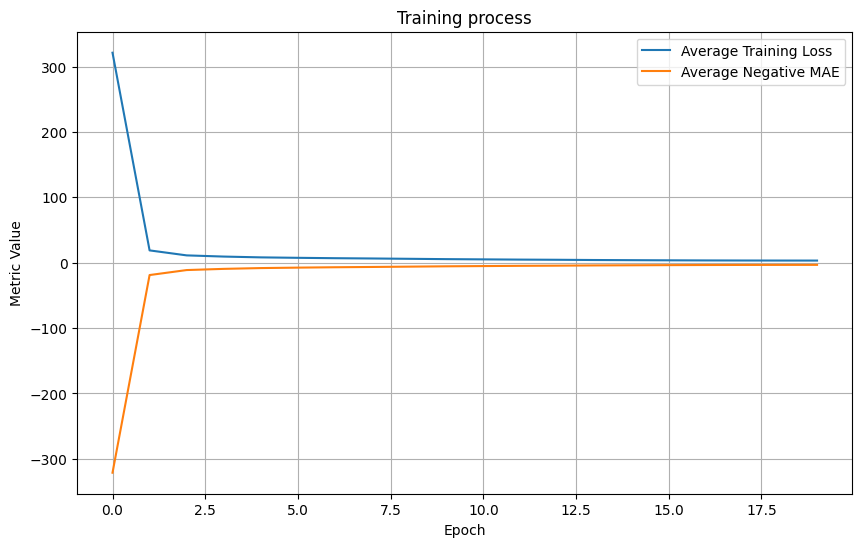
array([-321.24921668,  -18.86073489,  -11.22505361,   -9.40542923,
,        -8.18415683,   -7.5034998,   -6.91942925,   -6.48584448,
,        -5.98776587,   -5.48914804,   -5.12342416,   -4.76189905,
,        -4.50488674,   -4.14005336,   -3.90634942,   -3.68363947,
,        -3.51162539,   -3.39739157,   -3.32209207,   -3.28320729])
Conclution
In this project, I have used both machine learning and deep learning approaches to predict patient’s age based on EEG data.
The machine learning model provided an average MAE of 10.8 years. This means that on average, the model was about 10.8 years off from the actual age of the patient.
On the other hand, I implemented a deep learning model that achieved an MAE of 3.2 years(!). This means that on average, the deep learning model’s predictions were about 3.2 years off from the actual age.
Clearly, the deep learning model outperformed the machine learning model significantly.
However it’s important to note that the dataset I used for this project is relatively small, and I had limited computational resources available.
Therefore, while these results are promising, they should be taken cautiously. Further testing and validation on larger datasets and with more computational power would be necessary to confirm the effectiveness of these models.