Podcast topic suggestions using topic modeling and NLP
Topic modeling and natural language processing techniques to generate new topic ideas for a podcast
data scraping
visualisation
topic modeling
nlp
openai
Author
Shai Nisan
Published
May 9, 2023
This project involves using topic modeling and natural language processing techniques to generate new topic ideas for one of my favorite podcasts: Akimbo.
By analyzing a corpus of text data, the most common themes and topics are identified, and suggestions are made for potential podcast topics.
The project showcases the use of machine learning techniques to generate new ideas and provides a useful tool for content creators looking to diversify their podcast offerings.
import requestsfrom bs4 import BeautifulSoupimport pandas as pdimport numpy as npimport re, nltk, spacy, gensimimport matplotlib.pyplot as plt%matplotlib inlineimport seaborn as snsimport pprintimport matplotlib.patheffects as path_effectsfrom gensim.utils import simple_preprocessfrom gensim.models import LdaModelfrom gensim.corpora import Dictionaryfrom gensim.models import CoherenceModelfrom collections import Counterfrom nltk.corpus import stopwordsnltk.download('stopwords')nltk.download('wordnet')nltk.download('omw-1.4')nltk.download('averaged_perceptron_tagger')from nltk.stem import WordNetLemmatizerfrom wordcloud import WordCloud, STOPWORDS, ImageColorGeneratorfrom scipy.sparse import csr_matriximport pyLDAvisimport pyLDAvis.gensimimport gensim.corpora as corporafrom gensim.utils import simple_preprocessfrom gensim.models import CoherenceModel
[nltk_data] Downloading package stopwords to
[nltk_data]     C:\Users\nisan\AppData\Roaming\nltk_data...
[nltk_data]   Package stopwords is already up-to-date!
[nltk_data] Downloading package wordnet to
[nltk_data]     C:\Users\nisan\AppData\Roaming\nltk_data...
[nltk_data]   Package wordnet is already up-to-date!
[nltk_data] Downloading package omw-1.4 to
[nltk_data]     C:\Users\nisan\AppData\Roaming\nltk_data...
[nltk_data]   Package omw-1.4 is already up-to-date!
[nltk_data] Downloading package averaged_perceptron_tagger to
[nltk_data]     C:\Users\nisan\AppData\Roaming\nltk_data...
[nltk_data]   Package averaged_perceptron_tagger is already up-to-
[nltk_data]       date!
# Getting the data from the websiteresponse = requests.get("https://seths.blog/akimbo-podcast-transcripts/")soup = BeautifulSoup(response.content, "html.parser")# find all the text on the webpagetext = soup.get_text()# extract the chapter titles and textchapter_regex = re.compile(r"==>\s*(.+?)\s*<==")chapter_matches = chapter_regex.finditer(text)data = []for match in chapter_matches: chapter = match.group(1) text = match.string[match.end():].split("==>")[0].strip() data.append({"chapter": chapter, "text": text})# create a DataFrame from the extracted datadf = pd.DataFrame(data)df.head()
chapter
text
0
-paying-for-stamps-
Nobody tells a better story about ancient Rome...
1
-lots-of-questions-
The cool thing about knock knock jokes is that...
2
-queuing-theory-
Here’s a seemingly unrelated trivia question t...
3
-pay-the-writer-
37 years ago. I was in a jam. I had an idea fo...
4
-consolidation-publishing-
Newell Brands is a consumer facing conglomerat...
# Save it...df.to_csv('akimbo.csv', index=False)
# Load it...df = pd.read_csv('akimbo.csv')# Clean the chapter columndf["chapter"] = df["chapter"].str.replace("-"," ").str.strip()# Print some basic info about the textprint("* We have scraped", len(df), "chapters in the podcast.")print("\n* There are", round(df['text'].str.count(r'\w+').mean(), 1), "words in average per chapter.")print("\n* The longest chapter had", df['text'].str.count(r'\w+').max(), "words. \n It was chapter", df['text'].str.count(r'\w+').idxmax()+1, "with title: '"+df['chapter'].loc[df['text'].str.count(r'\w+').idxmax()].split(' ', 1)[1]+"'.")print("\n* The shortest chapter had", df['text'].str.count(r'\w+').min(), "words. \n It was chapter", df['text'].str.count(r'\w+').idxmin()+1, "with title: '"+df['chapter'].loc[df['text'].str.count(r'\w+').idxmin()].split(' ', 1)[1]+"'.")
* We have scraped 156 chapters in the podcast.

* There are 4298.4 words in average per chapter.

* The longest chapter had 10729 words.
  It was chapter 134 with title: 'season 7 opener'.

* The shortest chapter had 2210 words.
  It was chapter 76 with title: 'opportunity cost'.
# The fun part begins - preprocessing the data.# Get the text from the DataFrame and put it in a listdata =list(df.text)# Create bigrams from the databigram = gensim.models.Phrases(data, min_count=20, threshold=100)# Create trigrams from the bigramstrigram = gensim.models.Phrases(bigram[data], threshold=100)# Create a Phraser object from the bigram modelbigram_mod = gensim.models.phrases.Phraser(bigram)# Create a Phraser object from the trigram modeltrigram_mod = gensim.models.phrases.Phraser(trigram)
# load spacy model and disable parser and named entity recognitionnlp = spacy.load('en_core_web_sm', disable=['parser', 'ner'])# get stopwords from nltk librarystop_words = nltk.corpus.stopwords.words('english')def process_words(texts, stop_words=stop_words, allowed_tags=['NOUN', 'ADJ', 'VERB', 'ADV']):# remove stopwords, short tokens and letter accents texts = [[word for word in simple_preprocess(str(doc), deacc=True, min_len=3) if word notin stop_words] for doc in texts]# implement bigram and trigram models texts = [bigram_mod[doc] for doc in texts] texts = [trigram_mod[bigram_mod[doc]] for doc in texts] texts_out = []# implement lemmatization and filter out unwanted part of speech tagsfor sent in texts: doc = nlp(" ".join(sent)) texts_out.append([token.lemma_ for token in doc if token.pos_ in allowed_tags])# remove stopwords and short tokens again after lemmatization texts_out = [[word for word in simple_preprocess(str(doc), deacc=True, min_len=3) if word notin stop_words] for doc in texts_out] return texts_out
# convert text to preprocessed tokensdata_ready = process_words(data)# create a dictionary mapping tokens to idsid2word = corpora.Dictionary(data_ready)# print the total number of unique tokens in the dictionaryprint('Total Vocabulary Size:', len(id2word))
Total Vocabulary Size: 12554
corpus = [id2word.doc2bow(text) for text in data_ready]
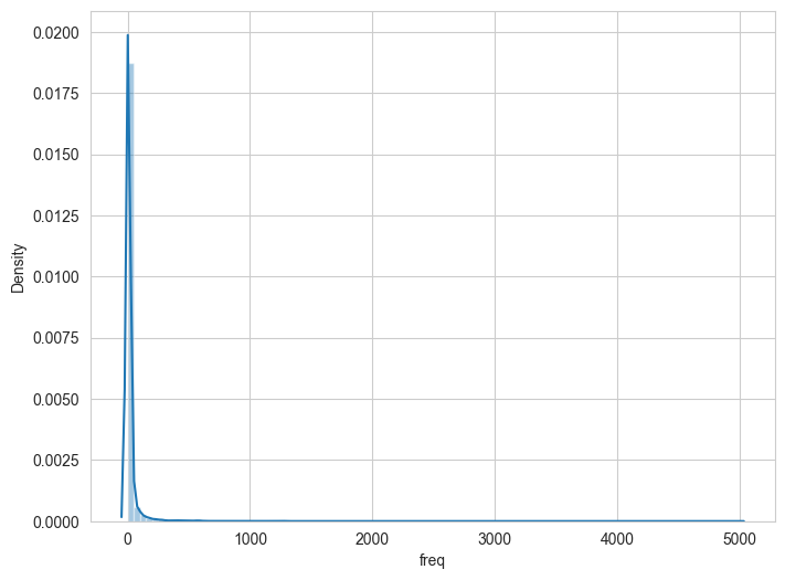
# create an empty dictionary to hold the word frequenciesdict_corpus = {}# loop through each document in the corpusfor i inrange(len(corpus)):# loop through each token and its frequency in the current documentfor idx, freq in corpus[i]:# check if the token is already in the dictionary, and update the frequency count accordinglyif id2word[idx] in dict_corpus: dict_corpus[id2word[idx]] += freqelse: dict_corpus[id2word[idx]] = freq# create a DataFrame from the dictionary of word frequencies dict_df = pd.DataFrame.from_dict(dict_corpus, orient='index', columns=['freq'])
# Creates a distribution plot for the frequency of the words in the corpus.plt.figure(figsize=(8,6))sns.distplot(dict_df['freq'], bins=100);
C:\Users\nisan\AppData\Local\Temp\ipykernel_21512\3304968696.py:3: UserWarning:

`distplot` is a deprecated function and will be removed in seaborn v0.14.0.

Please adapt your code to use either `displot` (a figure-level function with
similar flexibility) or `histplot` (an axes-level function for histograms).

For a guide to updating your code to use the new functions, please see
https://gist.github.com/mwaskom/de44147ed2974457ad6372750bbe5751

  sns.distplot(dict_df['freq'], bins=100);
# Sort the words in descending order by frequency and get the top 30 wordsdict_df.sort_values('freq', ascending=False).head(30)
freq
people
4984
get
4212
make
3151
work
2651
thing
2333
time
2246
want
2016
well
1981
say
1913
way
1840
know
1819
see
1767
question
1629
think
1546
idea
1273
year
1271
show
1266
really
1251
need
1219
book
1208
thank
1183
good
1141
come
1106
world
1093
talk
1084
take
1026
new
1006
first
972
change
956
right
954
# creates a list of words that have a frequency greater than 1500 in the corpusextension = dict_df[dict_df.freq>1500].index.tolist()
# add high frequency words to stop words liststop_words.extend(extension)# rerun the process_words functiondata_ready = process_words(data)# recreate Dictionaryid2word = corpora.Dictionary(data_ready)print('Total Vocabulary Size:', len(id2word))
Total Vocabulary Size: 12562
# Filter out words that occur less than 10 documents, or more than 50% of the documents.id2word.filter_extremes(no_below=10, no_above=0.5)print('Total Vocabulary Size:', len(id2word))
Total Vocabulary Size: 1828
# Create Corpus: Term Document Frequencycorpus = [id2word.doc2bow(text) for text in data_ready]
# Add it to the dfdf['processed_text'] = data_ready
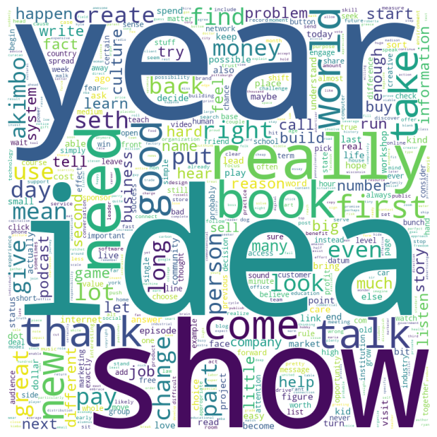
# Wordcloud of our corpus# Combine all documents into a single stringtext =' '.join([' '.join(doc) for doc in data_ready])# Count the occurrences of each wordword_counts = Counter(text.split())# Create wordcloudwordcloud = WordCloud(width=800, height=800, background_color='white', max_words=600).generate_from_frequencies(word_counts)# Display the generated image:plt.figure(figsize=(10, 6), facecolor=None)plt.imshow(wordcloud)plt.axis("off")plt.tight_layout(pad=0)plt.show()
c:\Users\nisan\AppData\Local\Programs\Python\Python310\lib\site-packages\wordcloud\wordcloud.py:106: MatplotlibDeprecationWarning: The get_cmap function was deprecated in Matplotlib 3.7 and will be removed two minor releases later. Use ``matplotlib.colormaps[name]`` or ``matplotlib.colormaps.get_cmap(obj)`` instead.
  self.colormap = plt.cm.get_cmap(colormap)
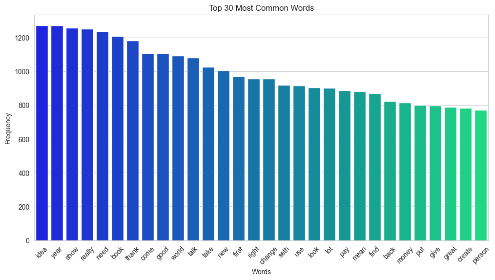
# Sort the words by their frequency in descending ordersorted_word_counts =sorted(word_counts.items(), key=lambda x: x[1], reverse=True)# Plot the top 30 wordsplt.figure(figsize=(12, 6))sns.set_style("whitegrid")sns.barplot(x=[word[0] for word in sorted_word_counts[:30]], y=[word[1] for word in sorted_word_counts[:30]], palette="winter")plt.xticks(rotation=45)plt.title("Top 30 Most Common Words")plt.xlabel("Words")plt.ylabel("Frequency")plt.show()
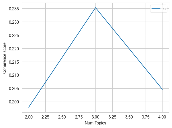
# A function that coputes coherence scores for different LDA modelsdef compute_coherence_values(dictionary, corpus, texts, limit, start=2, step=3): coherence_values = [] model_list = []for num_topics inrange(start, limit, step): model = LdaModel(corpus=corpus, id2word=id2word, num_topics=num_topics, random_state=0, chunksize=100, alpha='auto', per_word_topics=True) model_list.append(model) coherencemodel = CoherenceModel(model=model, texts=texts, dictionary=dictionary, coherence='c_v') coherence_values.append(coherencemodel.get_coherence())return model_list, coherence_valuesmodel_list, coherence_values = compute_coherence_values(dictionary=id2word, corpus=corpus, texts=data_ready, start=2, limit=5, step=1)# Show graph of the LDA modelslimit=5; start=2; step=1;x =range(start, limit, step)plt.plot(x, coherence_values)plt.xlabel("Num Topics")plt.ylabel("Coherence score")plt.legend(("coherence_values"), loc='best')plt.show()
# Get the model with the highest coherence valuebest_num_topics = x[np.argmax(coherence_values)]best_model = model_list[np.argmax(coherence_values)]# create function to get main topic for each documentdef get_main_topic(lda_model, doc):# get topic distribution for document topic_distribution = lda_model.get_document_topics(doc, minimum_probability=0.0)# sort topics by probability in descending order sorted_scores =sorted(topic_distribution, key=lambda x: x[1], reverse=True)# return index of topic with highest probabilityreturn sorted_scores[0][0]# apply LDA model to each document in dataframedf['doc'] = df['processed_text'].apply(lambda x: id2word.doc2bow(x))df['topic_LDA'] = df['doc'].apply(lambda doc: get_main_topic(best_model, doc))# display dataframedf.head()
chapter
text
processed_text
doc
topic_LDA
0
paying for stamps
Nobody tells a better story about ancient Rome...
[tell, story, ancient, rome, great, steve, pre...
[(0, 1), (1, 2), (2, 1), (3, 1), (4, 2), (5, 1...
1
1
lots of questions
The cool thing about knock knock jokes is that...
[cool, knock, knock, joke, always, answer, tod...
[(5, 2), (6, 1), (9, 1), (11, 1), (14, 1), (19...
1
2
queuing theory
Here’s a seemingly unrelated trivia question t...
[seemingly, unrelated, trivium, start, name, w...
[(6, 1), (8, 1), (12, 1), (13, 2), (19, 1), (2...
1
3
pay the writer
37 years ago. I was in a jam. I had an idea fo...
[year, ago, jam, idea, book, need, write, writ...
[(8, 2), (12, 1), (16, 1), (18, 1), (25, 1), (...
0
4
consolidation publishing
Newell Brands is a consumer facing conglomerat...
[newell, brand, consumer, face, conglomerate, ...
[(0, 1), (13, 1), (14, 2), (15, 1), (18, 1), (...
2
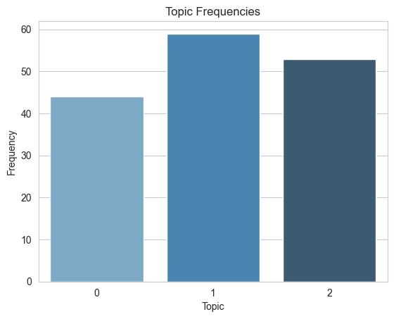
# Count the frequency of each topictopic_counts = df['topic_LDA'].value_counts()# Create bar plotsns.set_style("whitegrid")sns.barplot(x=topic_counts.index, y=topic_counts.values, palette="Blues_d")plt.title("Topic Frequencies")plt.xlabel("Topic")plt.ylabel("Frequency")plt.show()
# Visualize the model with pyLDAvisimport pyLDAvis.gensim_modelspyLDAvis.enable_notebook()vis = pyLDAvis.gensim_models.prepare(best_model, corpus, dictionary=id2word)vis
# Write the main topics from looking at pyLDAvis topics_list ="""The main topics for Akimbo Podcast are:***************************************Topic #0: Creativity.Topic #1: Marketing.Topic #2: Social Understanding."""print(topics_list)
The main topics for Akimbo Podcast are:
***************************************
Topic #0: Creativity.
Topic #1: Marketing.
Topic #2: Social Understanding.
# A helper function to prompt openai's apiimport openaiimport osopenai.api_key =''def get_completion(prompt, model="gpt-3.5-turbo"): messages = [{"role": "user", "content": prompt}] response = openai.ChatCompletion.create( model=model, messages=messages, temperature=0.5, )return response.choices[0].message["content"]
# Get recommendations for new podcast episodes for each topic based on the top keywordstopic_names = ["Creativity", "Marketing", "Social Understanding"]for i inrange(len(best_model.show_topics())): prompt =f""" Your task is to generate recommendations for the podcast episodes for this topic, with the help of the provided keywords. Write three recommendations for new episodes topics. Each recommendation should be a sentence with 3 to 8 words. Main keywords: {best_model.show_topics()[i]} """print(f"Recommendations for topic {i} - {topic_names[i]}:\n{get_completion(prompt)}\n")
Recommendations for topic 0 - Creativity:
1. "The Power of Placebo: Debunking Myths and Exploring Benefits"
2. "Leveraging Creative Marketing Strategies for Public Health Campaigns"
3. "Copyright Law and the Music Industry: Navigating Challenges and Opportunities"

Recommendations for topic 1 - Marketing:
1. "The Power of Creative Team Building"
2. "Perfecting Your Phone Etiquette"
3. "Building a Family-Run Business Model"

Recommendations for topic 2 - Social Understanding:
1. "Marketing Strategies for Difficult Industries"
2. "Effective Meeting Techniques for Productive Conversations"
3. "The Power of Attention: How to Pick the Right Target Audience"